Introduction

A basic way for the adaptation and constant modification of the learner’s experience of the real world is the process of Mathematical Modelling (MM), i.e. the solution of real world problems occurred in science and our everyday life situations.

MM appears today as a dynamic tool for teaching and learning mathematics, because it connects mathematics with the everyday life, thus giving the possibility to students to understand its usefulness in practice, and therefore increasing their interest about it.¹

In earlier works (e.g. ², ³: Chapters 5-7, etc) we have used several fuzzy logic techniques, like the measurement of a fuzzy system’s uncertainty, the Center of Gravity (COG) defuzzification technique and its variations, triangular and trapezoidal fuzzy numbers, etc, for assessing student MM skills and we have compared their outcomes with the outcomes of the traditional assessment methods of the bi-valued logic (average of student scores, GPA index, etc.).   

Here a new approach will be developed involving the use of Fuzzy Relation Equations (FRE) for evaluating the student MM skills. The rest of the paper is formulated as follows: The second Section contains the background from fuzzy binary relations and FRE which is necessary for the understanding of the paper. The original results of the paper are contained in the third Section, where the model using FRE for studying MM skills is developed. Those results are illustrated in the fourth Section with a classroom application and other suitable examples. Finally, the fifth Section is devoted to our conclusion and to some hints for future research on the subject.   

Fuzzy Relation Equations (FRE)

Fuzzy Logic, due to its nature of characterizing the ambiguous real life situations with multiple values, offers rich resources for handling problems with approximate data (e.g. see ,^4-7 etc.). This multiple-valued logic, being an extension / complement of the classical bi-valued Logic of Aristotle, is based on the notion of Fuzzy Set (FS), introduced by Zadeh in 1965 [8]. For general facts on FS we refer to the book.⁹

Definition 1: Let X, Y be two crisp sets. Then a fuzzy binary relation R(X, Y) is a FS on the Cartesian product X x Y of the form:

R(X, Y) = {(r, m_R(r): r = (x, y)  X x Y},

where m_R : X x Y [0, 1] is the corresponding membership function.-

When X = {x₁,…., x_n} and Y = {y₁,…, y_m}, then a fuzzy binary relation R(X, Y) can be represented by a n X m matrix of the form:

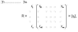
where rij = mR (xi, yj), with i = 1,…, n and j=1,…, m. The matrix R is called the membership matrix of the fuzzy relation R(X, Y).   
The basic ideas of fuzzy relations, which were introduced by Zadeh¹⁰ and were further investigated by other researchers, are extensively covered in the book.¹¹
Definition 2: Consider two fuzzy binary relations P(X, Y) and Q(Y, Z) with a common set Y. Then, the standard composition of these relations, which is denoted by P(X, Y)  Q(Y, Z), produces a a new binary relation R(X, Z) with membership function mR defined by
 
mR(xi, zj) =  min [mP(xi, y) , mQ(y, zj)]         (1)
for all i=1,…,n and all j=1,…,m. This composition is usually referred as the max-min composition.
Compositions of binary fuzzy relations are conveniently performed in terms of the membership matrices of those relations. In fact, if P = [pik] and Q=[qkj] are the membership matrices of the relations 
P(X, Y) and Q(Y, Z) respectively, then by relation (1) we get that the membership matrix of R(X, Y) = P(X, Y)  Q(Y, Z) is the matrix R = [rij], with 
rij =                                                           (2)

The same elements of P and Q are used in the calculation of R as it would be used in the regular multiplication of matrices, but the product and sum operations are here replaced with the min and max operations respectively.  
Definition 4: Consider the fuzzy binary relations P(X, Y), Q(Y, Z) and R(X, Z), defined on the sets, X = {xi : i  Nn} , Y = {yj : j  Nm }, Z= {zk : k  Ns}, where Nt = {1,2,…,t}, for t = n, m, k, and let P=[pij], Q=[qjk] and R=[rik] be the membership matrices of P(X, Y), Q(Y, Z) and R(X, Z) respectively. Assume that the above three relations constrain each other in such a way that 
P Q = R                                                    (3),
where “ ” denotes the max-min composition. This means that 
  min (p ij , q jk ) = rik                                (4),

for each i in Nn and each k in Ns. Therefore the matrix equation (3) encompasses n X k simultaneous equations of the form (4). When two of the components in each of the equations (4) are given and one is unknown, these equations are referred as fuzzy relation equations (FRE).
The notion of FRE was first proposed by Sanchez,¹² and later was further investigated by other researchers.^13-15

Assessment of MM Skills Using FRE
The process of MM involves the following steps: S1:  Analysis of the problem, S2: Mathematization (formulation of the problem and construction of the model), S3:  Solution of the model, S4:  Validation (control) of the model and implementation of the final mathematical results to the real system. (for more details see Section 2 of [2]). Without loss of generality the validation and the implementation of the model, which are usually considered as two different steps, have been joined here in one step in order to make simpler the development of our new assessment method
Let us consider the crisp sets X = {M}, Y = {A, B, C, D, F} and Z = {S1, S2, S3, S4}, where M denotes the “average student” of a class and A = Excellent, B = Very Good, C = Good, D = Satisfactory, F = Failed are the linguistic labels (grades) used for the assessment of the student performance .
Further, let n be the total number of students of a certain class and let ni be the number of students who obtained the grade i, i   Y. Then one can represent the average student of the class as a fuzzy set on Y in the form
M = {(i,  ): i  Y}.

The fuzzy set M induces a fuzzy binary relation P(X, Y) with membership matrix

P = [ ⁿA/n  ⁿB/n  ⁿC/n  ⁿD/n  ⁿF/n ]

In an analogous way the average student of a class can be represented as a fuzzy set on Z in the form

M = {(S_j, m(S_j): S_j Z},

where m: Z [0, 1] is the corresponding membership function. In this case the fuzzy set M induces a fuzzy binary relation R(X, Z) with membership matrix

R = [m(S₁) m(S₂)  m(S₃)  m(S₄)].

We consider also the fuzzy binary relation Q(Y, Z) with membership matrix the 5X4 matrix Q = [q_ij], where q_ij = m_Q(i, S_j) with i Y and S_j Z and the FRE encompassed by the matrix equation  (3), i.e. by PQ = R.

When the matrix Q is fixed and the row-matrix P is known, then the equation (3) has always a unique solution with respect to R, which enables the representation of the average student of a class as a fuzzy set on the set of the steps of the MM process. This is useful for the instructor for evaluating the performance of the class at each step of the MM process and therefore for designing his/her future teaching plans.

On the contrary, when the matrices Q and R, or P and R are known, then the equation (3) could have no solution or could have more than one solution with respect to P or Q respectively, which makes the corresponding situation more complicated.

The above remarks will be illustrated in the next section with a classroom application and other suitable examples.    

A Classroom Application and Other Examples

The Classroom Application

Table 1 depicts the results of a written test on MM problems performed on a group of freshmen students of the Graduate T. E. I. of Western Greece:

Table 1: Student Performance

Therefore, the average student M of the class can be represented as a fuzzy set on Y = {A, B, C, D, F} by 

M = {(A,  ), (B,  ), (C,  ), (D,  ), (F,  )}  {(A, 0.33), (B, 0.25), (C, 0.12), (D, 0.17), (F, 0.13)}

Thus M induces a fuzzy binary relation P(X, Y), where X = {M}, with membership matrix 

P = [0.33  0.25  0.12 0.17 0.13].

Also, using statistical data of the last five academic years  about the MM skills of the students of the Graduate TEI of Western Greece, we fixed the membership matrix Q of the fuzzy binary relation Q(Y, Z), where Z = {S₁, S₂, S₃, S₄}, in the form: 

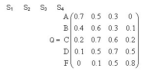
The statistical data used to form the matrix Q were collected by the instructor who was inspecting the student reactions during the solution of several MM problems in the classroom.Next, using the max-min composition of fuzzy binary relations one finds that the membership matrix of

R(X, Z) = P(X, Y) o Q (Y, Z) is equal to

R  =  P o Q  =  [0.33  0.33  0.3 0.17].

Therefore the average student of the class can be expressed as a fuzzy set on Z by

M = {(S₁, 0.33), (S₂, 0.33), (S₃, 0.3), (S₄, 0.17)}.

The conclusions obtained from the above expression of M are the following:

1. Only the  of the students of the class were ready to use contents of their memory (background knowledge, etc.) in order to facilitate the solution of the given problems.

2. All the above students designed successfully the model and almost all of them executed the solutions of the given problems.

3. On the contrary, half of the above students did not succeed to check the correctness of the solutions found and therefore to implement correctly the obtained mathematical results to the real system.

The first conclusion was not surprising, since the majority of the students have the wrong habit to start studying their courses the last month before the final exams. On the other hand, the second conclusion shows that the instructor’s teaching procedure was successful enabling the diligent students to plan and execute successfully the solutions of the given problems. Finally, the third conclusion is due to the fact that half of the students who had solved the given problems omitted to check if their solutions are compatible to the restrictions imposed by the real world (see Appendix). Therefore, it is very important for the instructor to emphasize that the last step of the MM process (checking and implementation) is not a formality, but it has its own importance for preventing several mistakes.

Other Examples

 Let us now consider the case where the membership matrices Q and R are known and we want to determine the matrix P representing the average student of the class as a fuzzy set on Y. This is a complicated case because we may have more than one solution or no solution at all. The following two examples illustrate this situation:

Example 1: Consider the membership matrices Q and R of the previous application and set

P = [p₁  p₂  p₃  p₄  p₅].

Then the matrix equation P o Q = R encompasses the following equations:

max {min (p_{1 ,} 0.7), min (p_2, 0.4), min (p_3, 0.2), min (p_4, 0.1), min (p₅, 0)}= 0.33

max {min (p_{1 ,} 0.5), min (p_2, 0.6), min (p_3, 0.7), min (p_4, 0.5), min (p₅, 0.1)}= 0.33

max {min (p_{1 ,} 0.3), min (p_2, 0.3), min (p_3, 0.6), min (p_4, 0.7), min (p₅, 0.5)}= 0.3

max {min (p_{1 ,} 0), min (p_2, 0.1), min (p_3, 0.2), min (p_4, 0.5), min (p₅, 0.8)}= 0.17

The first of the above equations is true if, and only if, p₁ = 0.33 or p₂ = 0.33, values that satisfy the second and third equations as well. Also, the fourth equation is true if, and only if, p₃ = 0.17 or p₄ = 0.17 or p₅ = 0.17. Therefore, any combination of values of p₁, p₂, p₃, p₄, p₅ in [0, 1] such that p₁ = 0.33 or p₂ = 0.33 and p₃ = 0.17 or p₄ = 0.17 or p₅ = 0.17 is a solution of P o Q = R.

 Let S(Q, R) = {P: P o Q = R } be the set of all solutions of P o Q = R. Then one can define a partial ordering on S(Q, R) by

P P΄   p_i  p΄_i, ι = 1, 2, 3, 4, 5.

It is well known that whenever S(Q, R) is a non empty set, it always contains a unique maximal solution and it may contain several minimal solutions.¹⁶ It is further known that S(Q, R) is fully characterized by the maximal and minimal solutions in the sense that all its other elements are between the maximal and each of the minimal solutions.¹⁶ A method of determining the maximal and minimal solutions of P o Q = R with respect to P has been developed in.¹⁸   

Example 2: Let Q = [q_ij], i = 1, 2, 3, 4, 5 and j = 1, 2, 3, 4 be as in Example 2 and let R = [1 0.33 0.3 0.17]. Then the first equation encompassed by the matrix equation P o Q = R is

max {min (p_{1 ,} 0.7), min (p_2, 0.4), min (p_3, 0.2), min (p_4, 0.1), min (p₅, 0)}= 1

In this case it is easy to observe that the above equation has no solution with respect to p₁, p₂, p₃, p₄, p₅, therefore P o Q = R has no solution with respect to P.

In general, writing R = {r₁ r₂  r₃  r₄}, it becomes evident that we have no solution  if  max q_ij < r_j .  j

With analogous to the above examples one can show that, if the membership matrices P and R are known, then the equation (3) can have no solution, or more than one solutions with respect to Q.

Conclusion

In the present article we used principles of the theory of FRE to build up a model for evaluating student MM skills. More explicitly, the point-by-point process followed is the introduction to the theory of FRE through the fuzzy binary relations, the use of their principles on the steps of the MM process (analysis, mathematization, solution, validation / implementation) to construct our model and the applications developed to illustrate it in practice. 

In this way we have managed to express the “average student” of a class as a fuzzy set on the set of the steps of the MM process, which gives valuable information to the instructor for designing his future teaching plans. On the contrary, we have realized that the problem of representing the “average student” of a class as a fuzzy set on the set of the linguistic grades characterizing his or her performance using FRE is complicated, since it may have more than one solutions or no solution at all.

In general, the use of FRE looks as a powerful tool for the assessment of human skills and therefore our future research plans include the effort of using them for a better description and assessment of other human activities apart from the MM process, like learning, reasoning, computational thinking, decision-making, sports and games, etc.

References

- Voskoglou M.Gr. Mathematical Modelling as a Teaching Method of Mathematics, Journal for Research in Innovative Teaching (National University, CA, USA). 2015;8(1):35-50.
- Voskoglou M.Gr. Fuzzy Logic, Computers and Mathematical Modelling, Transactions on Mathematics. 2017;3(2):14-26.
- Voskoglou M.Gr. Finite Markov Chain and Fuzzy Logic Assessment Models: Emerging Research and Opportunities, Columbia, SC: Createspace.com. – Amazon. 2017.
- Arqub A.O., Abo-Hamour Z. Numerical solution of systems of second-order boundary value problems using continuous genetic algorithm, Information Sciences. 2014;279:396-415.
CrossRef - Arqub A.O., Al-Smadi M., Momani S. Numerical solutions of fuzzy differential equations using reproducing kernel Hilbert space method, Soft Computing. 2016;20(8):3283-3302.
CrossRef - Arqub A.O., Al-Smadi M., Momani S. Application of reproducing kernel algorithm for solving second-order, two-point fuzzy boundary value problems, Soft Computing. 2017;21(23):7191-7206.
CrossRef - Arqub A. O. Adaptation of reproducing kernel algorithm for solving fuzzy Fredholm-Volterra integrodifferential equations, Neural Computing & Applications. 2017;28(7):1591-1610.
CrossRef - Zadeh L. A. Fuzzy sets, Information and Control. 1965;8:338-353.
CrossRef - Klir G. J., Folger T. A. Fuzzy Sets, Uncertainty and Information, New Jersey: Prentice-Hall. 1988.
- Zadeh L. A. Similarity relations and fuzzy orderings, Information Sciences. 1971;3:177-200.
CrossRef - Kaufmann A. Introduction to the Theory of Fuzzy Subsets, New York: Academic Press. 1975
- Sanchez E. Resolution of Composite Fuzzy Relation Equations, Information and Control. 1976;30:38-43.
CrossRef - Czogala E., Drewniak J., Pedryz W. Fuzzy relation equations on a finite set, Fuzzy Sets and Systems. 1982;7:89-101.
CrossRef - Higashi M., Klir G. J. Resolution of finite fuzzy relation equations, Fuzzy Sets and Systems. 1984;13:65-82.
CrossRef - Prevot, M., Algorithm for the solution of fuzzy relations, Fuzzy Sets and Systems. 1981;5:319-322.
CrossRef
This work is licensed under a Creative Commons Attribution 4.0 International License.